In my last post on computer vision and memorability, I looked at an already existing model and started experimenting with variations on that architecture. The most successful attempts were those that use Residual Neural Networks. These are a type of deep neural network built to mimic specific visual structures in the brain. ResMem, one of the new models, uses a variation on ResNet in its architecture to leverage that optical identification power towards memorability estimation. M3M, another new model, extends this even further by also including semantic segmentation data generated by another Residual Neural Network based method, but more on that later.

ResMem

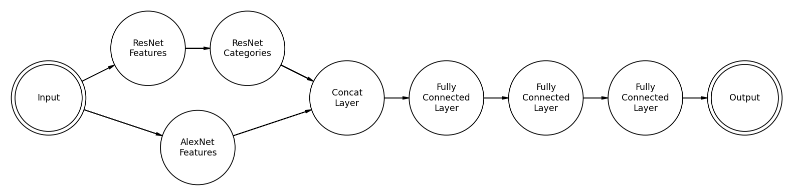
Above is a skeleton diagram of the ResMem architecture. We put an image in the input, which has been cropped and resized to 227x227. We feed that image to both an AlexNet-style feature space, a convolutional neural network, and the ResNet categorizer, which outputs a vector of 1000 numbers between 0 and 1. The output of the AlexNet feature space takes the form of 256 channels with size 6x6. The model then rearranges this output into a 1D vector of size 9216. The “Concat layer” then combines these into one vector of size 10216. The model runs that vector through a series of fully connected layers. The skeleton diagram shows three layers, but the published version contains six fully connected layers before the output layer. We transform that output with a sigmoid function, and it turns into a memorability score.

What, though, is the logic behind each of these design choices? Why split the image across different kinds of feature decompositions? We tend to think that because a technology is derived from an older technology, the new one is strictly better. This is not precisely true in the case of ResNet vs. AlexNet. The benefit of using ResNet is that it allows extremely deep neural networks. On the other hand, AlexNet has fewer layers. Having more layers leads to more abstract information, which leads to better inference. AlexNet has fewer layers, so the features it outputs are more concrete. This gets into the fundamental theoretical difference between ResMem and ResMemRetrain. ResMem’s ResNet features are the abstract category vector. That is what ResNet was built for. ResMemRetrain, however, has reoptimized that feature vector for memorability. This limits our chances to interpret any features but improves the model’s accuracy. When the ResNet and AlexNet feature spaces are combined, this gives the fully connected section access to both concrete and abstract features in making the final prediction.

And it does! Adding the ResNet features improves rank correlation from the 0.45 range to the 0.6 range. Training time on my 1080TI is about 30 minutes for ResMem and an hour and a half for ResMemRetrain. My laptop can make inferences on a set of 10000 images in about ten minutes. In other words, we do sacrifice a lot of simplicity for this accuracy boost, but it’s absolutely manageable; for contrast, let’s consider M3M.

M3M

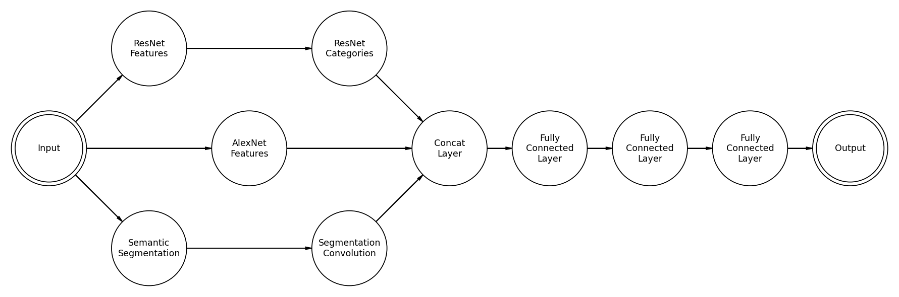
The main difference here is that we added a semantic segmentation feature. Semantic segmentation is a way to infer a label for every pixel in an image. Generally, this technique is used for things like self-driving cars.

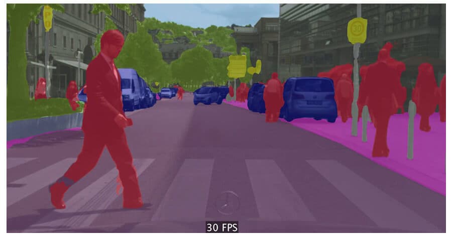
The image above is an example of a semantic segmentation output. You see, it does good enough, but there is some misassignment around the borders of objects. Here’s the problem, to mix this back into the fully connected layer, we can’t just unwrap the image with category assignment into a vector; it would be huge. It would take more memory than most GPUs have to store the weight vector for the first fully connected layer. There are 13 categories, and the image is 227x227, so that means it’s a vector of length 669,877, adding in the ResNet and AlexNet features it’s 680,093. The first fully connected layer has an output space of size 4096. That gives us 2,785,660,928 weights. Each weight is stored as a 32 bit float, so the weight tensor is 89,141,149,696 bits, 11,142,643,712 bytes, or 11.14 GB. Just barely too big for my 1080TI, and too big for most GPUs.¹

But I digress. The solution to this convolution problem is, of course, more convolution. So M3M runs the semantic segmentation output through another couple of convolution layers and then feeds that into the fully connected block.

What does this convoluted mess actually do for us? M3M gets rank correlations on the order of 0.67 in validation, so there’s a noticeable improvement. But at what cost? M3M has ~500M parameters. Compared to ResMem’s 70M, M3M takes about six times as long to train. In other words, I don’t think it’s worth it. Besides, M3M takes up about 2GB of VRAM, which is manageable for most graphics cards, but it’s not exactly “portable.” And that’s just the parameters, torch stores a lot more than only the parameters, so you usually end up with a model size about twice that figure. 4GB is pushing it for a model to run on anyone’s computer. So since the actual increase in accuracy that we get from adding semantic segmentation information is marginal, we may as well stick with ResMem.